Coordinating protection without time grading
Two devices in series on a radial feeder see the same fault. The conventional way to decide which one clears it is to separate their curves in time: the upstream device waits a coordination interval longer than the downstream one, and selectivity follows.
It works. It is also the only discriminant available that is paid for in conductor damage, arc energy and customers who felt the sag.
Time is a finite resource on a feeder, and the conventional scheme spends it in exactly the wrong place. The device with the longest delay is the one standing where the fault current is highest.
This is about the alternatives: what else can carry the discrimination, what each one requires, and how to work out which the feeder in front of you needs.
Where the time lives in the equation
Start with the machinery, because the constraint is visible in it. IEEE C37.112 defines the inverse-time characteristic as:
where is the operating time in seconds, the time dial, the fault current, the pickup setting, and , and the constants that fix the curve shape:
| Curve | A | B | p |
|---|---|---|---|
| Moderately inverse | 0.0515 | 0.1140 | 0.02 |
| Very inverse | 19.61 | 0.4910 | 2 |
| Extremely inverse | 28.20 | 0.1217 | 2 |
Three degrees of freedom per element and no more: positions the curve horizontally, scales it vertically, and the constant set fixes its shape. is worth noticing on its own: it is a horizontal asymptote, the floor the curve approaches as grows. IEC 60255-151 has no equivalent term, which is why an IEC very-inverse and an IEEE very-inverse diverge at high current despite sharing a name.
The standard also defines a reset characteristic, which gets skipped more often than it should:
It emulates the mechanical inertia of an induction disc. On a feeder with reclosing, the reset mode decides whether an upstream device keeps or loses its integration between successive trips, and that turns out to be the root of a failure mode we will get to.
Why time runs out
Conventional coordination requires, for every fault current both devices can see:
The interval is not a safety factor, it is a sum: interrupting time of the downstream device (50–80 ms), relay overtravel, characteristic and instrument tolerance, and margin. Two to three hundred milliseconds on a numerical scheme.
That interval accumulates. With devices in cascade the head-end device carries roughly of inherited delay, and it carries it at the point of maximum available fault current. Four levels at 0.3 s puts the substation breaker near a second for a fault on its own bus.
Four distinct limits show up in practice:
- Accumulation. Described above. Bites hardest at moderate currents, where the inverse term still dominates.
- No current contrast. On a short or stiff feeder, barely changes between adjacent devices, so both curves are evaluated at nearly the same multiple and only can separate them.
- Identical curves in series. The normal condition for line reclosers shipped with the same default configuration. Two identical curves do not coordinate at all: they operate together.
- Reclosing sequences. Fast and slow curves, operation counters and dead times introduce state that a curve pair does not describe. Two devices in series can drift out of sequence with each other.
Limits 3 and 4 are the important ones, because no amount of adjustment fixes either.
How much time is actually available
Worth doing the arithmetic once, because the intuition is usually wrong in both directions.
The thermal ceiling for a bare aluminium conductor follows the classic ICEA form, with in circular mils, from 90 °C operating to 340 °C annealing:
with in circular mils, operating and annealing.
For a 266.8 MCM ACSR trunk that gives , or 2.03 s at a 10 500 A bus fault. A 20 MVA substation transformer at 8 % impedance, checked against IEEE C57.109, gives essentially the same answer: 1.98 s.
So roughly two seconds, and that number is almost never the binding constraint. Two others are far tighter:
- Incident energy scales linearly with clearing time. Going from 0.4 s to 0.15 s cuts it to 37 %, which moves PPE categories.
- Voltage sag propagates to the whole substation bus, so a fault on one feeder is seen by every customer on all of them. The ITIC envelope tolerates 70 % voltage for about half a second; below 50 %, roughly 0.2 s.
The ceiling permits two seconds. Safety and power quality ask for less than 0.3 s. That gap is the entire motivation for what follows.
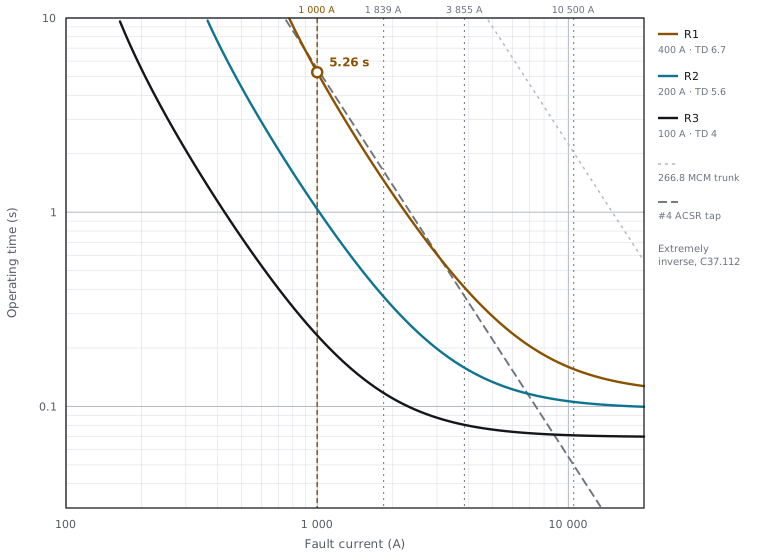
There is also a trap in the thermal check itself: the limit that matters is the smallest conductor inside the device's zone, not the trunk. The same formula gives a #4 ACSR tap only 0.37 s at 3 855 A, a limit a head-end setting of 0.41 s already violates, while the trunk sits comfortably at 15 s.
A reference feeder
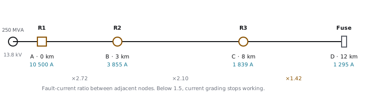
Concrete numbers make the comparisons meaningful. A 13.8 kV radial, 250 MVA at the bus, 266.8 MCM ACSR trunk at :
| Node | Distance | Device | I_cc (3φ) | Ratio to previous |
|---|---|---|---|---|
| A | 0 km | R1 (head) | 10 500 A | n/a |
| B | 3 km | R2 | 3 855 A | 2.72 |
| C | 8 km | R3 | 1 839 A | 2.10 |
| D | 12 km | Fuse | 1 295 A | 1.42 |
Conventional settings, extremely inverse throughout, :
| Device | I_pickup | TD fast | TD slow |
|---|---|---|---|
| R1 | 400 A | n/a | 6.7 |
| R2 | 200 A | 1.0 | 5.6 |
| R3 | 100 A | 1.0 | 4.0 |
Margins verify cleanly: 0.250 s at node C, 0.252 s at node B. The study passes.
Now evaluate the same settings at a 1 000 A fault: a high-impedance ground fault, or a fault near the end of the line under minimum generation:
| Device | t at 1 000 A |
|---|---|
| R3 | 0.232 s |
| R2 | 1.037 s |
| R1 | 5.26 s |
Five seconds of backup on a scheme whose coordination table shows no violations. The CTI check verifies selectivity. It says nothing about speed.
Four alternative discriminants
1. Current grading
Discriminate with instead of . Set the upstream instantaneous element so its reach stops short of the next device:
For R2 in the reference feeder that is 2 300 A. Solving places the reach at 6.09 km from the substation, 3.09 km past R2, covering 62 % of the R2–R3 section. A fault at 4 km clears in 0.030 s instead of 0.188 s, cutting by a factor of 6.
Validity condition is a ratio, and it is checkable before anything else:
In the reference feeder that holds for A–B and B–C and fails for C–D. The ratios predict which sections can be solved this way before a single setting is computed. This costs nothing and should always be the first check.
The limitations are real: no coverage of high-impedance faults, a dead zone at the end of the reach, and sensitivity to source strength variation.
2. Counting operations
Two mechanisms, both of which drop time comparison entirely.
Sequence coordination solves the identical-curves problem. Consider R2 and R3 with the same fast/slow sequence and a permanent fault below R3:
| Operation | R3 curve | R2 curve | t R3 | t R2 |
|---|---|---|---|---|
| 1 | fast (TD=1) | fast (TD=1) | 0.035 s | 0.090 s |
| 2 | fast (TD=1) | fast (TD=1) | 0.035 s | 0.090 s |
| 3 | slow (TD=4) | fast (TD=1) | 0.142 s | 0.090 s |
By the third operation R3 has advanced to its slow curve while R2, which never tripped, is still on fast. The margin is −0.051 s: R2 operates first and takes out everything upstream for a fault that belonged to R3.
The fix is for the upstream device to detect fault current followed by its extinction, and advance its own sequence counter without tripping. Both devices then reach operation 3 on their slow curves, and the margin becomes +0.364 s. No communications, no curve changes: the discriminant is the operation count. Vendors name this differently; NOJA Power calls it Zone Sequence Coordination.
Temporary time addition attacks accumulation from the other side. Instead
of separating the curves permanently, add a delay to the upstream device only
while a downstream isolation is in progress. In the reference feeder, dropping
R1 from TD = 6.7 to 3.0 with a 0.30 s temporary addition still satisfies
the node B requirement (0.484 s available against 0.408 s needed) while cutting
the bus-fault clearing time from 0.156 s to 0.070 s, and the 1 000 A case from
5.26 s to 2.65 s. The margin exists only when it is needed.
Sectionalisers remove curve comparison altogether. The device counts fault current pulses followed by loss of voltage and opens during the upstream dead time, without interrupting fault current. The setting window is:
For the C–D section, the one whose current ratio ruled out current grading, that gives 120 A ≤ ≤ 680 A, so 160 A with two counts. A new sectionalising point that consumes no time step at all.
The dependency is absolute: if the upstream device fails to interrupt, there is no local backup. Using a recloser in sectionaliser mode keeps interrupting capability in reserve, which is a meaningful advantage over a dedicated sectionaliser.
3. Logic selectivity
The downstream device signals a block on pickup; the upstream device trips instantaneously if no block arrives within a fixed window.
Time still exists, but it stops scaling with the number of levels. For a fault at node B, between R1 and R2, a 60 ms window (25 ms pickup + 5 ms GOOSE transmission + 30 ms margin) plus interrupting time clears in 0.13 s against 0.410 s on the curve. Incident energy falls by a factor of three.
The communications question deserves a straight answer, because it decides whether this is available at all. The criterion is not inside or outside the substation. It is a latency budget:
A 60–100 ms window needs tail latency below roughly 50 ms. That leaves:
| Medium | Typical latency | Verdict |
|---|---|---|
| Fibre (OPGW/ADSS) + GOOSE | 1–4 ms | Works, in the substation and on the line |
| Dedicated licensed point-to-point radio | 10–40 ms, load-dependent jitter | Marginal. Measure it, do not trust the datasheet |
| Cellular, DNP3 over private APN, multipoint SCADA radio | 100 ms to seconds | No. That is telemetry, not teleprotection |
Reusing the SCADA telemetry path for a blocking scheme is the failure mode to name explicitly. And the loss-of-channel behaviour matters: a blocking scheme degrades by over-tripping upstream. Safe for plant, destructive to reliability indices. Channel supervision and automatic reversion to the time-delayed curve are mandatory, not optional.
Schemes that operate on a scale of seconds, such as loop automation and automatic transfer, tolerate slow channels precisely because they are restoration schemes rather than protection.
4. Direction and topology
With distributed generation the discriminant becomes the angle, not the magnitude or the delay. A 3 MVA synchronous machine at node C with contributes:
For a fault at node B, R3 sees 837 A in the reverse direction against a 100 A pickup, and trips for a fault outside its zone. No value of prevents this because the reverse current legitimately exceeds pickup. Directional supervision, or setting groups switched by topology state, are the answer.
Choosing
An order of evaluation that reflects what each option costs:
| Approach | Discriminant | Communications | Cost | Validity condition |
|---|---|---|---|---|
| Current grading | Magnitude | No | None | Ratio ≳ 1.5 between nodes |
| Sequence coordination | Operation count | No | Firmware | Similar curves in series |
| Temporary time addition | Conditional delay | No | Firmware | Recloser cascade |
| Sectionaliser | Event count | No | None to low | Reliable upstream device |
| Logic blocking | Logic signal | Yes | Medium to high | Supervised channel |
| Directional / groups | Angle, state | Optional | Low | Voltage reference, study |
The first four require no communications infrastructure and are enabled by parameterisation of equipment that is often already installed. That is where to start.
If this is being automated, the useful structure is a hierarchy rather than a weighted score. Thermal damage of every element in zone, interrupting duty and minimum-fault sensitivity are hard constraints. Incident energy is next. Coordination interval after that. Sag duration and reliability indices become the objective function. And the infeasibility of the coordination problem is itself the most valuable signal a study produces: it is the point at which the answer stops being a different and starts being a different scheme.
Closing
The habit worth breaking is reaching for the time dial first. It is the most visible knob and the one every study is built around, but it is also the only discriminant whose price is paid in damage, in arc energy and in customers who noticed.
Selectivity bought with current, with counting or with logic costs essentially nothing. Selectivity bought with time is charged to the feeder.
Sources
On the numbers in this article. Every value in the reference feeder is computed, not quoted: the operating times come from the IEEE C37.112 equation printed above, the thermal limits from the ICEA formula printed above, and the coordination margins are their differences. They can be reproduced with a calculator from the tables given. Spot-checking a few: R1 at 10 500 A gives 0.156 s and at 1 000 A gives 5.26 s; the 266.8 MCM trunk gives , or 2.03 s at the bus fault, while the #4 tap gives 0.37 s at 3 855 A.
On the standards. The following are the documents that govern this material, and where the curve constants, the through-fault limits and the arc-flash method come from:
| Standard | Covers |
|---|---|
| IEEE C37.112 | Inverse-time characteristic equations |
| IEC 60255-151 | Over/undercurrent protection, curve equations |
| IEEE C37.230 | Protective relay applications to distribution lines |
| IEEE C57.109 | Transformer through-fault duration guide |
| IEEE Std 242 | Protection and coordination (the Buff Book) |
| IEEE 1584 | Arc-flash hazard calculation |
| IEEE C37.2 | Device function numbers |
I did not open these standards while writing this. They are paywalled and I do not hold current copies. The constants in the curve table, the ICEA coefficient and the ITIC envelope figures are quoted from working knowledge, and anyone using them for an actual setting calculation should take them from the standard itself rather than from this page. What this article does stand behind is the arithmetic built on top of them and the argument about which discriminant costs what.
On the vendor feature named in the text. Zone Sequence Coordination is NOJA Power's name for the operation-counting scheme described in section 2; other vendors implement the same idea under other names. I did not consult that vendor's documentation for this article, and the behaviour described is the generic mechanism, not a specification of any particular product.
Unstated inputs, declared. Two figures in the text depend on inputs the article does not give: the sectionaliser window of 120 A to 680 A implies a load current and a minimum fault current for the C–D section that are not listed in the feeder table, and the 6.09 km reach depends on solving the impedance model for distance. Both are internally consistent with the stated feeder, but a reader cannot re-derive them from the tables alone.